Google Sheets VLOOKUP for Beginners

The fundamental purpose of the VLOOKUP in Google Sheets is to do a vertical search, where it looks for a specific key value (unique identifier) in the first column of a given range and then finds and returns the corresponding value from another column in the same row.

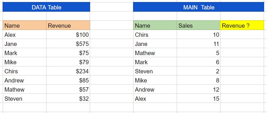
Now let's learn using a real example - here, we want to match the revenue of each salesperson in the MAIN table with the revenue in the DATA table.

Back to basics!

Below is the syntax for Google Sheets Lookup Function:

=VLOOKUP(search_key, range, index, [is_sorted])

search_key - is the key value we search, here its Name

range - is two or more columns of data for the search, here it's the data table.

index - is the column number of the data we want to match, here it's 1 (the revenue column)

is_sorted - FALSE = Exact match and TRUE = Approximate match. It's important to opt for FLASE to properly match the data in the vlookup

Let's Start!

STEP 1

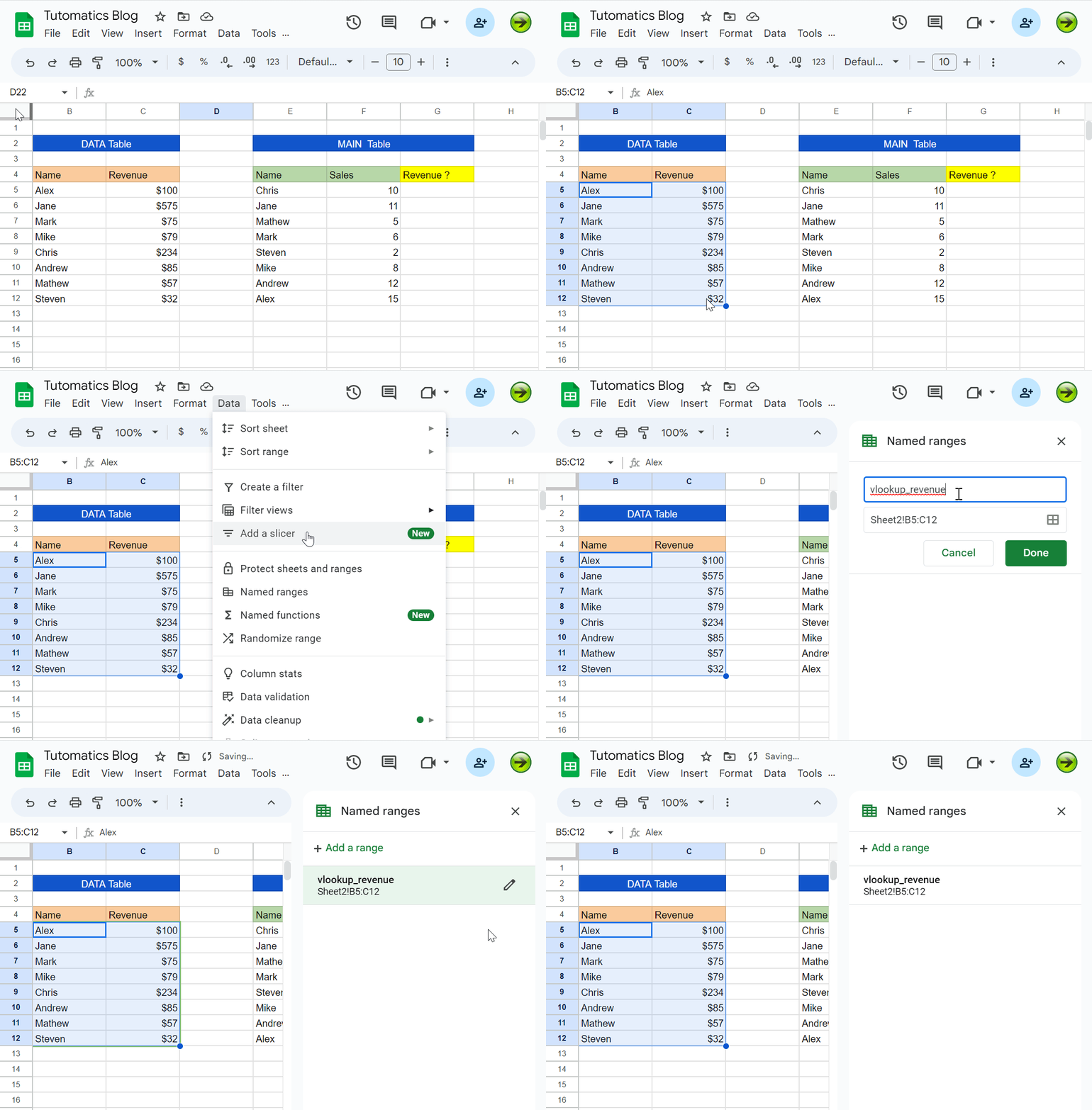
As the first step, create the range of data; you can do this by dragging the data without the headers and clicking on DATA > NAMED RANGES

And give it a name, I used vlookup_revenue here

STEP 2

Lets write the formula for row 1

=VLOOKUP(E5, vlookup_revenue, 2, false)

1. Here E5 is the row associated with the first name of my table, which is Chris.
2. vlookup_revenue - is the lookup data we created in STEP 1
3. 2 - is the column number of the revenue column which we need to match
4. false - we use this option to exactly match the values in Lookup

STEP 3

Copy and paste the formula across (or accept auto-suggestion) the column, and you are done!